Suppose you created a table in Excel, and you want to add a column in it. In that case, What will you do? Simply go to your Excel worksheet and add a new column to it. But this column will not be added to your Pivot Table. Then, How do you edit or delete in Pivot Table?
The Pivot Table is an easy way to summarize data from the worksheet or an external source. You can calculate totals, averages, counts, etc. in any numeric field in your table. You can also create charts from your tables.
Look at the below tables:


See the difference when you go to Pivot Table.

Nothing is changed because you change in the original table, not in Pivot Table. If you want to change in Pivot Table you have to use the Refresh Button.
What is Refresh Button?
You can use the refresh button to refresh the field value. Following are the steps to use the Refresh button to refresh your column value:
- Go to the Pivot Table, it is on the same worksheet or another worksheet.
- Click anywhere in the Pivot Table area. Two tabs appear: Analyze and Design. (If you clicked outside the Pivot Table area, these two options will not appear).Click on the Analyze tab, then select the Refresh button.

- There is a change in a field value, as you can see.

How to Show New Added Column in Pivot Table?
Let’s say you want to add a new column to your table.
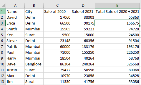
If you go and Refresh your Pivot Table, a new column does not appear because you change in your table, not in Pivot Table. Here, the Refresh button is not working because you add a new column.
To show the newly added column you should follow the following steps:
- Go to the Pivot Table worksheet (it is on the same worksheet or another).
- Once you have clicked anywhere in the Pivot Table area, two tabs will appear. Analyze and Design. (If you clicked outside the Pivot Table area, these two options will not appear). Click on Analyze Tab. Then click Change Data Source.

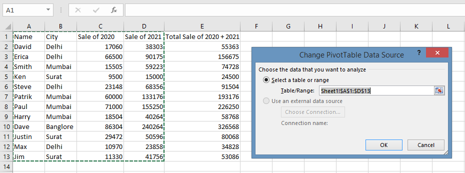
Your newly created column will not be selected in the range and picks up the old columns by default.
- You must now select the range of the table either manually (typing the range in the text box) or automatically (doing drag button).

- Then click the Ok button.
- There is a new field in the PivotTable Fields appear.
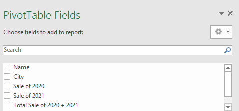
- Now, you can also select the Total Sales of 2020 + 2021.
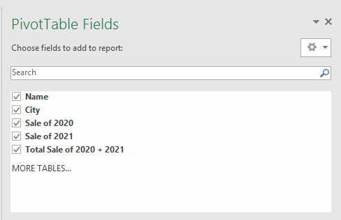
- Below is the result.

Remove Pivot Table Fields Value
When you want to delete your Pivot Table data, choose the Clear Option.
- Go to the Pivot Table worksheet. (It is on the same sheet or some other sheet.)
- Click anywhere in the Pivot Table area. Two tabs will appear. Analyze and Design. (If you click outside Pivot Table, these two options will not appear). Click on Analyze Tab. Click on the Clear Option.

- Choose the option Clear All.
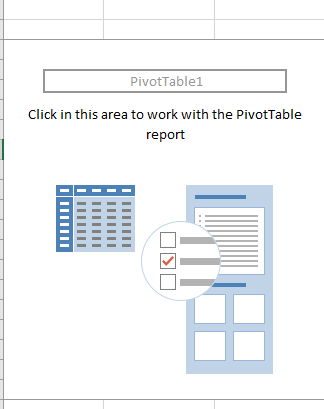
This will clear all Pivot Table items but not the structure.
Delete Structure of Pivot Table
To delete the structure of the Pivot Table you can do the following things:
- First, you have to delete the field value by using the Clear All button.
- You will see two tabs. Analyze and Design (If you click outside the Pivot Table area, these options will not appear). Click on the Analyze Tab. Click on Select and then Entire Pivot Table.
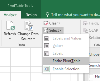
- The Pivot Table is selected.

- Then go to the Home Tab and select Clear All Option.

- Pivot Table structure is deleted. As shown in below:
